Contemplating LayerNorm

Centering around mean centering

A detail about LayerNorm has always been confusing to me, hearing about RMSNorm¹ finally prompted me to write about it.

Batch Normalization (BatchNorm)² is applied to a minibatch of activation vectors. It mean-centers the vectors, using the mean vector over the minibatch, then (elementwise) re-scales by the (elementwise) standard deviation. This is meant to combat covariate shift during training.

\(\begin{align*} \vec{\mu} &= \sum_{i=1}^k \vec{x}^{(i)} / k \\ \vec{\sigma} &= \sqrt{\sum_{i=1}^k (\vec{x}^{(i)} - \vec{\mu})^2 / k} \\ \vec{y}^{(i)} &= \frac{\vec{x}^{(i)}-\vec{\mu}}{\vec{\sigma}} \end{align*}\)

(Square, square-root of a vector, and division of a vector by another is elementwise, 𝑖 indexes an element of the minibatch of size 𝑘.)

Layer Normalization (LayerNorm)³ simplifies this and makes it applicable to a single vector. It “mean-centers” the vectors, using the mean scalar over the vector, then (elementwise) re-scales by the scalar standard deviation over the vector.

\(\begin{align*} \mu &= \sum_{j=1}^D \vec{x}_j / D \\ \sigma &= \sqrt{\sum_{j=1}^D (\vec{x}_j - \mu)^2/D} \\ \vec{y} &= \frac{\vec{x}-\mu}{\sigma} \end{align*}\)

(𝑗 indexes an element of a vector with 𝐷 dimensions.)

The interesting distinction here is that 𝜇 and 𝜎 are scalars. Since mean and stdev are computed over the dimensionality 𝑗, there is no need for the index 𝑖 here, so it can apply to a single vector (a minibatch of size 1).

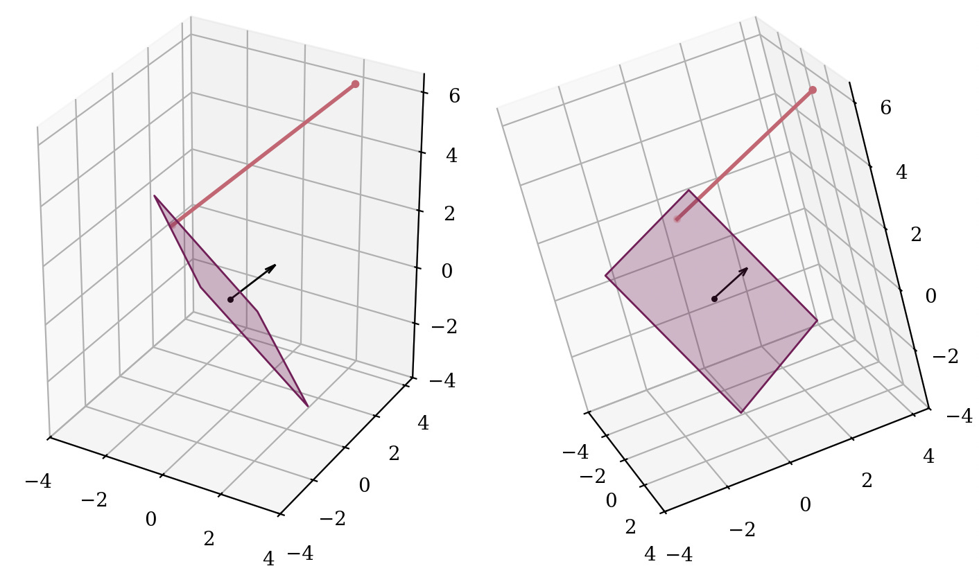
I wanted to better understand what this operation did. What does “mean-centering” part look like here? We subtract a scalar 𝜇 from the vector 𝑥, which is the same as subtracting 𝜇·𝟏 if 𝟏 denotes the all-ones vector. Thus, we translate 𝑥 along the direction of 𝟏 = [1, …, 1]. Note that this vector is the normal vector of the hyperplane 𝑥₁ + … + 𝑥ₙ = 𝑐 for any 𝑐. Furthermore, after the translation, the sum 𝑥₁ + … + 𝑥ₙ will always equal 0, simply because of how much we translate (which is 𝜇):

\(\begin{align*} \sum_j(\vec{x}_j-\mu) &= \sum_j x_j - D \mu \\ &= \sum_j x_j - D \frac{\sum_j x_j}{D} \\ &= \sum_j x_j - \sum_j x_j\\ &= 0 \end{align*}\)

Thus, the “mean-centering” is exactly the act of projecting 𝑥 onto the 𝑥₁ + … + 𝑥ₙ = 0 hyperplane.

Projection of the point [2, 4, 6] (pink) onto the aforementioned hyperplane shown from two angles. Result is the point [-2, 0, 2]. Violet square is a segment of the hyperplane. Black arrow shows the normal vector [1, 1, 1] (anchored at the origin).

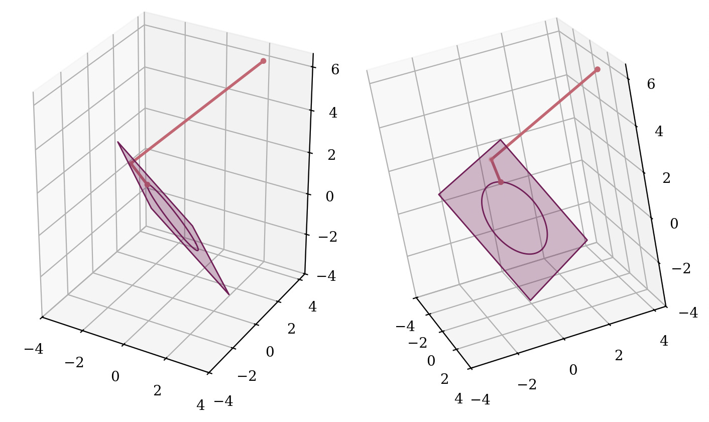
Afterwards, the mean-centered vector is re-scaled such that it has variance over vector elements is 1. This keeps the direction of the vector, and scales it to have a Euclidean norm of √𝐷. Therefore, this is projecting onto the sphere with radius √𝐷. A detail here is that we were already in the (𝐷-1)-dimensional hyperplane, therefore we can only arrive at the (𝐷-1)-dimensional slice of the 𝐷-dimensional sphere.

Previous point on the hyperplane is projected once more, this time onto the √3-scaled circle on the hyperplane. Final point is ~[-1.225, 0, 1.225] lying on the violet circle.

This second part is relatively easy to motivate, keeps the direction, keeps the norm contained and under control for the downstream layers, and so on. However the first part seems peculiar… Why do we want to project onto 𝑥₁ + … + 𝑥ₙ = 0 first? This seems like an additional loss in the degree of freedom (or dimensionality) without much gain. The norm might not shrink that much if the vector is already close to the hyperplane, and can still be arbitrarily large. And we are going to project onto the sphere later anyways, so why also have this step? The direction of [1, …, 1] seems arbitrary, is there a reason to think that this particular hyperplane or normal vector has a special impact? Could we project onto any other (𝐷-1)-dimensional hyperplane crossing the origin?

Invariance analysis section in the LayerNorm paper shows one invariance this mean-centering brings in: Invariance to weight matrix re-centering by a constant row-vector. Adding the same row-vector to each row of a weight matrix results in each linear unit to shift by the same scalar (i.e., along [1, …, 1]), which is nullified by such mean-centering. However this feels a bit like kicking down the can, as it is not obvious to me how the learning dynamics could cause a weight matrix drift by approximately constant row-vectors, so it is merely pushing the same question further down. Although, I can see this easily happen with something like a sum over hidden units, which would backpropagate the same scalar gradient to each hidden unit. On the other hand, we wouldn’t apply mean-centering to such layers anyways because it makes the sum a constant function. 🤔

Mean-centering typically invokes connotations about placing a clump of points such that they are spread about the origin. However, as we see, mean-centering the scalar values of a single vector has a very different behavior compared to this intuition. To re-emphasize, below are plots of three clusters of data (left), mean-centered BatchNorm-style (middle) and LayerNorm-style (right) (only the mean-centering part applied, excludes the re-scaling):

Left: Three clusters of points (violet, pink, orange). Middle: Mean-centered using vectorwise mean per cluster (BatchNorm). Right: Mean-centered using scalarwise mean per vector (LayerNorm). Top: Angled looking sideways to the 𝑥₁ + 𝑥₂ + 𝑥₃ = 0 plane (azimuth = -30). Bottom: Angled looking across the 𝑥₁ + 𝑥₂ + 𝑥₃ = 0 plane (azimuth = 60).

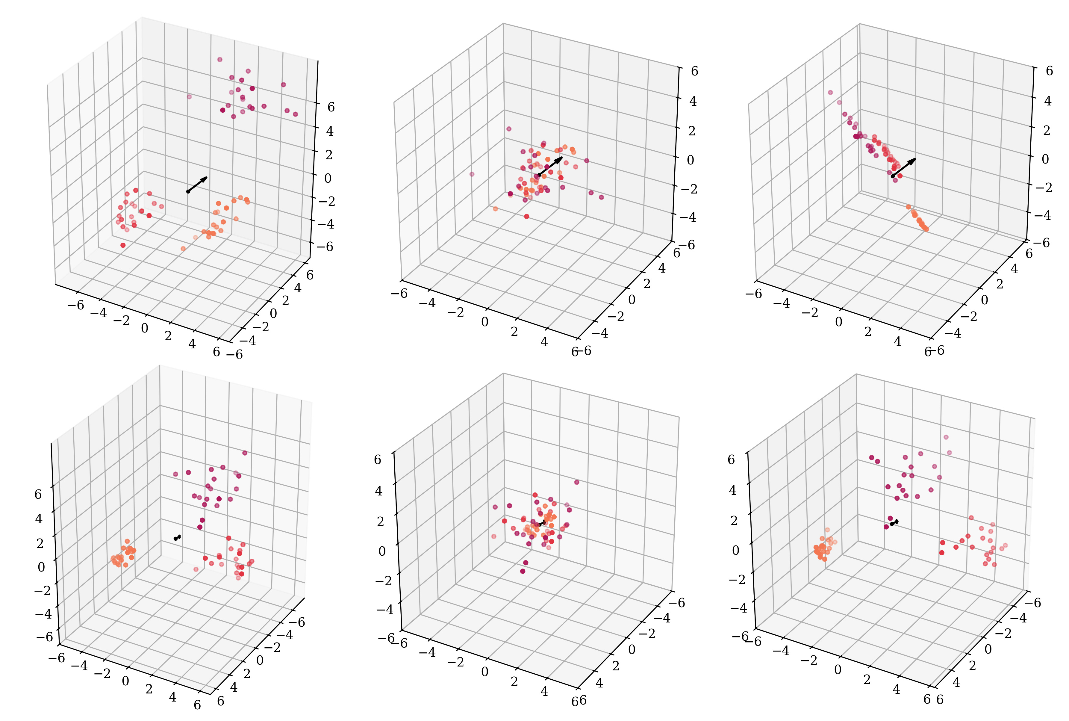
In the top right, we see the points lying flat on the same 2d-plane. In the bottom right when we look across the same hyperplane, we do observe clusters (minibatches) away from, and not centered around, the origin.

Is this merely a mismatch of intuition and desiderata? If scalarwise mean-centering is not well motivated, could we just skip that and jump directly to the normalization? I wish I had acted on this question in time 😅, but some researchers apparently tried exactly this and proposed RMSNorm. They do seem to suggest that, at least empirically, the mean-centering part of LayerNorm might not be needed. I don’t know if the authors motivated their work from a similar start, as I did not find a geometric interpretation of the function in their paper, so I decided to write this post to share my own thoughts.

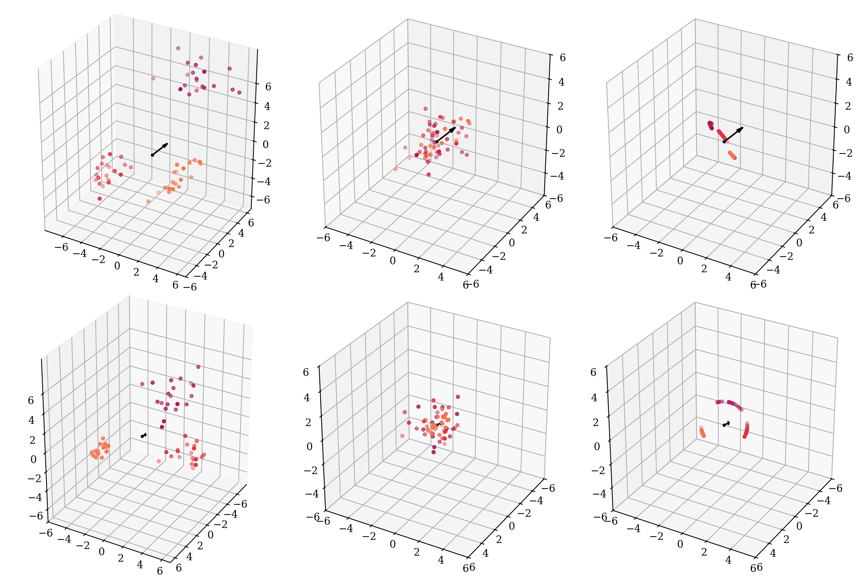
Appendix: Extra figures

Same cluster of points (left) applied BatchNorm (middle) and LayerNorm (right) including the re-scaling step. Top: Angled looking sideways to the 𝑥₁ + 𝑥₂ + 𝑥₃ = 0 plane (azimuth = -30). Bottom: Angled looking across the 𝑥₁ + 𝑥₂ + 𝑥₃ = 0 plane (azimuth = 60).

Same toy projection example, with RMSNorm added (orange), which shows what would happen if we were to directly apply RMS norm step after skipping mean-centering, projecting the original point onto the √3-scaled sphere.

1. B. Zhang, R. Sennrich. Root Mean Square Layer Normalization. https://arxiv.org/abs/1910.07467

2. S. Ioffe, C. Szegedy. Batch Normalization: Accelerating Deep Network Training by Reducing Internal Covariate Shift. https://arxiv.org/abs/1502.03167

3. J. L. Ba, J. R. Kiros, G. E. Hinton. Layer Normalization. https://arxiv.org/abs/1607.06450